The goal of inteRact is to make affect control theory (ACT) equations accessible to a broader audience of social scientists.
ACT is a theory of social behavior that rests upon a control process in which people act in ways that maintain cultural meaning. ACT theoretical concepts have been fruitful when applied to research within cultural sociology (Hunzaker 2014, 2018), stratification and occupational prestige (Freeland and Hoey 2018), social movements (shuster and Campos-Castillo. 2017), and gender and victimization (Boyle and McKinzie 2015; Boyle and Walker 2016). Information about ACT as a theory can be accessed here: https://research.franklin.uga.edu/act/
The goal of this package is to make elements of typical ACT analyses easier to implement into R: calculating the deflection of an event, the optimal behavior of an actor after an event, the relabeling of the actor or object after an event, and calculating emotions within events. You can look within the functions to see how the equations were programmed, but to truly get a handle on the equations and how they work, I refer you to Expressive Order (Heise 2010).
Installation
You can install the development version from GitHub with:
# install.packages("devtools")
devtools::install_github("ekmaloney/inteRact")
Example Analysis
The following analysis is an example of how to use this package to implement ACT equations in your work. Because interact.jar is an excellent Java program intended for the use of examining single events in great detail, inteRact privileges workflows that intend to apply Affect Control Theory equations to many events at once. Functions can still be applied to one event, but the steps required to apply the functions may seem onerous for only one single event.
First, for any analysis you do, you need to ensure that the identities, behaviors, and modifiers that you study are measured in an ACT dictionary. inteRact requires the use of an accompanying data package, actdata, maintained by Aidan Combs and accessible here (https://github.com/ahcombs/actdata). In the following analysis, I will be using the most recent US dictionary, the US Full Surveyor Dictionary collected in 2015.
The first step in an analysis is to create a data frame of events - these events should follow the actor-behavior-object format of a typical ACT interaction. This data frame can either be wide (a column each for actor, behavior, and object), or long (multiple rows per event).
library(inteRact)
#> Loading required package: actdata
library(actdata)
library(tidyverse)
#> ── Attaching packages ─────────────────────────────────────── tidyverse 1.3.1 ──
#> ✓ ggplot2 3.3.5     ✓ purrr   0.3.4
#> ✓ tibble  3.1.6     ✓ dplyr   1.0.7
#> ✓ tidyr   1.1.4     ✓ stringr 1.4.0
#> ✓ readr   2.1.1     ✓ forcats 0.5.1
#> ── Conflicts ────────────────────────────────────────── tidyverse_conflicts() ──
#> x dplyr::filter() masks stats::filter()
#> x dplyr::lag()    masks stats::lag()

#get US 2015 dictionary using the epa subset from the actdata package
us_2015 <- epa_subset(dataset = "usfullsurveyor2015")

#make a dataframe of events
set.seed(369)
events_wide <- tibble(actor = sample(us_2015$term[us_2015$component == "identity"], 10),
                 behavior = sample(us_2015$term[us_2015$component == "behavior"], 10),
                 object = sample(us_2015$term[us_2015$component == "identity"], 10))

set.seed(369)
events_long <- tibble(id = rep(1:10, 3),
                      term = c(sample(us_2015$term[us_2015$component == "identity"], 10),
                               sample(us_2015$term[us_2015$component == "behavior"], 10),
                               sample(us_2015$term[us_2015$component == "identity"], 10)),
                      element = rep(c("actor", "behavior", "object"), each = 10)) %>%
                arrange(id)

head(events_wide)
#> # A tibble: 6 × 3
#>   actor      behavior  object
#>   <chr>      <chr>     <chr>
#> 1 landlady   fluster   introvert
#> 2 virgin     shield    neurotic
#> 3 chatterbox educate   myself_as_i_would_like_to_be
#> 4 shop_clerk entreat   best_man
#> 5 grind      aggravate machine_repairer
#> 6 asian_man  berate    chatterbox
head(events_long)
#> # A tibble: 6 × 3
#>      id term      element
#>   <int> <chr>     <chr>
#> 1     1 landlady  actor
#> 2     1 fluster   behavior
#> 3     1 introvert object
#> 4     2 virgin    actor
#> 5     2 shield    behavior
#> 6     2 neurotic  object
The next step is to augment your events with the corresponding EPA measures from the ACT dictionary. To do this, you should use the reshape_events_df on your events dataframe. You must indicate the dictionary you are using by its actdata key (in this case “usfullsurveyor2015”) and the gender of those dictionary estimates (here I am using the average of the male and female estimates). This function has an indicator whether your events dataframe is wide or long - if it is long, you must use the id_column argument to indicate the variable that you are using to group the events by.
analysis_df <- reshape_events_df(df = events_wide,
                                 df_format = "wide",
                                 dictionary_key = "usfullsurveyor2015",
                                 dictionary_gender = "average")
#> Joining, by = c("term", "component")

head(analysis_df)
#> # A tibble: 6 × 7
#>   event_id event                      element term  component dimension estimate
#>      <int> <chr>                      <chr>   <chr> <chr>     <chr>        <dbl>
#> 1        1 landlady fluster introvert actor   land… identity  E             0.08
#> 2        1 landlady fluster introvert actor   land… identity  P             1.68
#> 3        1 landlady fluster introvert actor   land… identity  A             0.59
#> 4        1 landlady fluster introvert behavi… flus… behavior  E            -0.32
#> 5        1 landlady fluster introvert behavi… flus… behavior  P             1.2
#> 6        1 landlady fluster introvert behavi… flus… behavior  A             0.81

analysis_df <- reshape_events_df(df = events_long,
                                 df_format = "long",
                                 id_column = "id",
                                 dictionary_key = "usfullsurveyor2015",
                                 dictionary_gender = "average")
#> Joining, by = c("term", "component")

head(analysis_df)
#> # A tibble: 6 × 7
#> # Groups:   event_id [1]
#>   term     element  component event_id event                  dimension estimate
#>   <chr>    <chr>    <chr>        <int> <chr>                  <chr>        <dbl>
#> 1 landlady actor    identity         1 landlady fluster intr… E             0.08
#> 2 landlady actor    identity         1 landlady fluster intr… P             1.68
#> 3 landlady actor    identity         1 landlady fluster intr… A             0.59
#> 4 fluster  behavior behavior         1 landlady fluster intr… E            -0.32
#> 5 fluster  behavior behavior         1 landlady fluster intr… P             1.2
#> 6 fluster  behavior behavior         1 landlady fluster intr… A             0.81
After reshaping your events, you now have a dataframe with the fundamental sentiments of each element of your Actor-Behavior-Object events. In ACT, fundamental sentiments are the stable cultural meaning of a social identity, behavior, or emotion. These sentiments fall along 3 dimensions: Evaluation, how good or bad the concept is, Potency, how powerful or weak, and Activity, how fast/young or slow/old. Values of these dimensions range from -4.3 (extremely bad, weak, slow) to 4.3 (extremely good, powerful, active).
Once you have the overall analysis dataframe, you should group_by the event_id and nest the rest of the data, this will allow you to apply the main ACT functions to each event in the dataframe. Next, you should add a column indicating the equation you will be using to analyze the events. This should take the form “{equation_key}_{gender}” from the actdata package. In the following code, you will see that I am using the us2010 equation averaged across genders to match the dictionary.
nested_analysis_df <- analysis_df %>%
                      group_by(event_id, event) %>%
                      nest() %>%
                      mutate(eq_info = "us2010_average")
Now, you can apply various functions to each event by using the map2() function from the purrr package. For example, to get the deflection of each event, you use the map2 function to iteratively apply the get_deflection function to each dataframe of events and equation information inside the nested dataframe.
results_df <- nested_analysis_df %>%
              mutate(deflection = map2_dbl(data, eq_info, get_deflection))

results_df %>% select(event, deflection)
#> Adding missing grouping variables: `event_id`
#> # A tibble: 10 × 3
#> # Groups:   event_id, event [10]
#>    event_id event                                           deflection
#>       <int> <chr>                                                <dbl>
#>  1        1 landlady fluster introvert                           2.18
#>  2        2 virgin shield neurotic                               6.93
#>  3        3 chatterbox educate myself_as_i_would_like_to_be     20.5
#>  4        4 shop_clerk entreat best_man                          0.994
#>  5        5 grind aggravate machine_repairer                    17.1
#>  6        6 asian_man berate chatterbox                         20.9
#>  7        7 crybaby harass sleuth                               19.8
#>  8        8 street_musician glorify mugger                       1.86
#>  9        9 chaplain chastise scoundrel                         22.8
#> 10       10 artist like newcomer                                12.2
Deflection
When applying Affect Control Theory in research contexts, one of the most typical questions is - what is the deflection of this event? The deflection is an indicator of how culturally unlikely an event is to occur - a higher deflection indicates a more unexpected event. ACT calculates how much each element (Actor, Behavior, Object) moves along each dimension (Evaluation, Potency, Activity) after an event - these new locations in EPA space are termed the transient impressions. The deflection is the sum of squared differences between the fundamental sentiments and transient impressions for each element of the event.
You can replicate the results from the get_deflection function by calculating the transient impression of each event, calculating the squared differences between fundamental sentiments and transient impressions, squaring them, and then summing those squared differences.
nested_analysis_df %>%
    mutate(trans_imp = map2(data, eq_info, transient_impression)) %>%
    unnest(trans_imp) %>%
    mutate(difference = estimate - trans_imp,
           sqd_difference = difference^2) %>%
    group_by(event_id, event) %>%
    summarise(deflection = sum(sqd_difference))
#> `summarise()` has grouped output by 'event_id'. You can override using the `.groups` argument.
#> # A tibble: 10 × 3
#> # Groups:   event_id [10]
#>    event_id event                                           deflection
#>       <int> <chr>                                                <dbl>
#>  1        1 landlady fluster introvert                           2.18
#>  2        2 virgin shield neurotic                               6.93
#>  3        3 chatterbox educate myself_as_i_would_like_to_be     20.5
#>  4        4 shop_clerk entreat best_man                          0.994
#>  5        5 grind aggravate machine_repairer                    17.1
#>  6        6 asian_man berate chatterbox                         20.9
#>  7        7 crybaby harass sleuth                               19.8
#>  8        8 street_musician glorify mugger                       1.86
#>  9        9 chaplain chastise scoundrel                         22.8
#> 10       10 artist like newcomer                                12.2
Element Deflection
You may even be particularly interested in which element-dimensions move the most in EPA space from your events.
nested_analysis_df %>%
    mutate(elem_def = map2(data, eq_info, element_deflection)) %>%
    unnest(elem_def) %>% ggplot(mapping = aes(x = sqd_diff)) +
      geom_histogram(binwidth = 0.5) + facet_grid(dimension ~ element) +
      theme_minimal() + labs(x = "Squared Difference between Fundamental and Transient")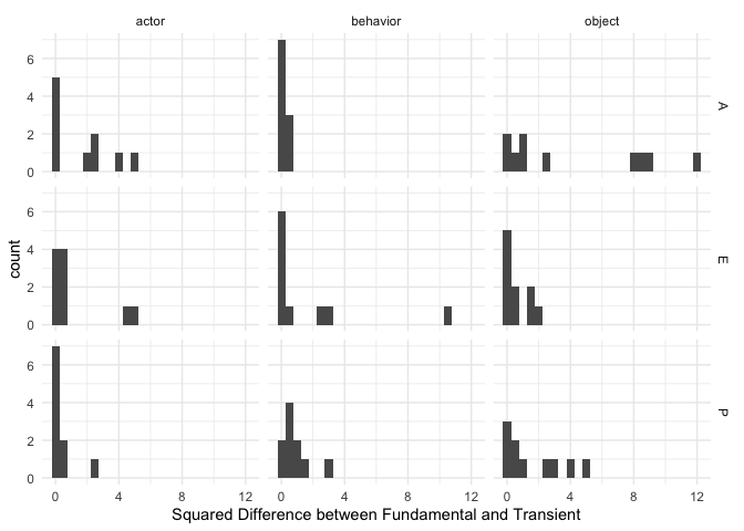
Optimal Behavior
ACT can also predict the optimal behavior for the actor to enact in the following interaction that would bring the transient sentiments back as close as possible to the fundamental sentiments. The function optimal_behavior finds the E, P, and A value for the optimal behavior
nested_analysis_df %>%
  mutate(opt_beh = map2(data, eq_info, optimal_behavior)) %>%
  unnest(opt_beh)
#> # A tibble: 20 × 8
#> # Groups:   event_id, event [10]
#>    event_id event               data     eq_info     opt_E   opt_P   opt_A term
#>       <int> <chr>               <list>   <chr>       <dbl>   <dbl>   <dbl> <chr>
#>  1        1 landlady fluster i… <tibble… us2010_a…  0.784   1.53    0.0992 actor
#>  2        1 landlady fluster i… <tibble… us2010_a…  0.393  -0.299  -1.94   obje…
#>  3        2 virgin shield neur… <tibble… us2010_a…  0.605   0.733  -1.05   actor
#>  4        2 virgin shield neur… <tibble… us2010_a… -0.983  -0.217   0.225  obje…
#>  5        3 chatterbox educate… <tibble… us2010_a… -0.0298 -0.274   2.78   actor
#>  6        3 chatterbox educate… <tibble… us2010_a…  1.37    2.59    1.58   obje…
#>  7        4 shop_clerk entreat… <tibble… us2010_a…  0.583   0.0312  0.319  actor
#>  8        4 shop_clerk entreat… <tibble… us2010_a…  0.784   1.60    0.431  obje…
#>  9        5 grind aggravate ma… <tibble… us2010_a…  0.201  -0.622   0.819  actor
#> 10        5 grind aggravate ma… <tibble… us2010_a…  0.753   2.12    0.741  obje…
#> 11        6 asian_man berate c… <tibble… us2010_a…  1.56   -0.0484  0.398  actor
#> 12        6 asian_man berate c… <tibble… us2010_a…  0.299   1.47    2.81   obje…
#> 13        7 crybaby harass sle… <tibble… us2010_a…  1.67   -0.889   1.70   actor
#> 14        7 crybaby harass sle… <tibble… us2010_a…  0.102   0.467  -1.75   obje…
#> 15        8 street_musician gl… <tibble… us2010_a… -0.0732 -0.114   1.62   actor
#> 16        8 street_musician gl… <tibble… us2010_a… -1.21    0.234   0.688  obje…
#> 17        9 chaplain chastise … <tibble… us2010_a…  1.59    1.19   -0.385  actor
#> 18        9 chaplain chastise … <tibble… us2010_a…  0.359   0.170   1.77   obje…
#> 19       10 artist like newcom… <tibble… us2010_a… -0.411   1.04   -0.696  actor
#> 20       10 artist like newcom… <tibble… us2010_a…  0.0461  0.303  -1.33   obje…
Actor and Object Reidentification
Following an ABO event, Actors and Objects can be reidentified by the other or an onlooker, to an identity that “fits” with their behavior better. The functions reidentify_actor and reidentify_object calculate this for you:
nested_analysis_df %>%
  mutate(new_actor_id = map2(data, eq_info, reidentify_actor),
         new_object_id = map2(data, eq_info, reidentify_object)) %>%
  unnest(new_actor_id)
#> # A tibble: 10 × 8
#> # Groups:   event_id, event [10]
#>    event_id event           data     eq_info        E     P      A new_object_id
#>       <int> <chr>           <list>   <chr>      <dbl> <dbl>  <dbl> <list>
#>  1        1 landlady flust… <tibble… us2010_a…  0.275 1.27   1.06  <tibble [1 ×…
#>  2        2 virgin shield … <tibble… us2010_a…  0.262 2.65   1.03  <tibble [1 ×…
#>  3        3 chatterbox edu… <tibble… us2010_a…  1.15  2.79  -0.277 <tibble [1 ×…
#>  4        4 shop_clerk ent… <tibble… us2010_a…  1.01  0.376 -0.250 <tibble [1 ×…
#>  5        5 grind aggravat… <tibble… us2010_a… -1.69  0.645  2.70  <tibble [1 ×…
#>  6        6 asian_man bera… <tibble… us2010_a… -2.90  0.756  2.86  <tibble [1 ×…
#>  7        7 crybaby harass… <tibble… us2010_a…  0.480 0.428  2.35  <tibble [1 ×…
#>  8        8 street_musicia… <tibble… us2010_a…  0.578 0.850  1.52  <tibble [1 ×…
#>  9        9 chaplain chast… <tibble… us2010_a… -2.84  0.904  1.89  <tibble [1 ×…
#> 10       10 artist like ne… <tibble… us2010_a… -1.02  1.60   0.185 <tibble [1 ×…
Closest Term
To find the closest measured identity, modifier, or behavior to an EPA profile, you can use the function closest_term which has 5 arguments: the E, P, and A measurements, the type of term (identity, modifier, or behavior, and the maximum distance away in EPA units the term can be).
nested_analysis_df %>%
  mutate(new_actor_id = map2(data, eq_info, reidentify_actor),
         new_object_id = map2(data, eq_info, reidentify_object)) %>%
  unnest(new_actor_id) %>%
  rowwise() %>%
  mutate(term = closest_term(E, P, A, dictionary_key = "usfullsurveyor2015", gender = "average",
               term_typ = "identity", num_terms = 1)) %>%
  unnest(cols = c(term))
#> # A tibble: 10 × 13
#> # Groups:   event_id, event [10]
#>    event_id event     data   eq_info      E     P      A new_object_id term_name
#>       <int> <chr>     <list> <chr>    <dbl> <dbl>  <dbl> <list>        <chr>
#>  1        1 landlady… <tibb… us2010…  0.275 1.27   1.06  <tibble [1 ×… grind
#>  2        2 virgin s… <tibb… us2010…  0.262 2.65   1.03  <tibble [1 ×… milliona…
#>  3        3 chatterb… <tibb… us2010…  1.15  2.79  -0.277 <tibble [1 ×… judge
#>  4        4 shop_cle… <tibb… us2010…  1.01  0.376 -0.250 <tibble [1 ×… rancher
#>  5        5 grind ag… <tibb… us2010… -1.69  0.645  2.70  <tibble [1 ×… speeder
#>  6        6 asian_ma… <tibb… us2010… -2.90  0.756  2.86  <tibble [1 ×… madman
#>  7        7 crybaby … <tibb… us2010…  0.480 0.428  2.35  <tibble [1 ×… busybody
#>  8        8 street_m… <tibb… us2010…  0.578 0.850  1.52  <tibble [1 ×… flirt
#>  9        9 chaplain… <tibb… us2010… -2.84  0.904  1.89  <tibble [1 ×… bully
#> 10       10 artist l… <tibb… us2010… -1.02  1.60   0.185 <tibble [1 ×… mafioso
#> # … with 4 more variables: term_E <dbl>, term_P <dbl>, term_A <dbl>, ssd <dbl>